


Introduction
Reinforcement Learning (RL) refers to both the learning problem and the sub-field of machine learning which has lately been in the news for great reasons. RL based systems have now beaten world champions of Go, helped operate datacenters better and mastered a wide variety of Atari games. The research community is seeing many more promising results. With enough motivation, let us now take a look at the Reinforcement Learning problem.
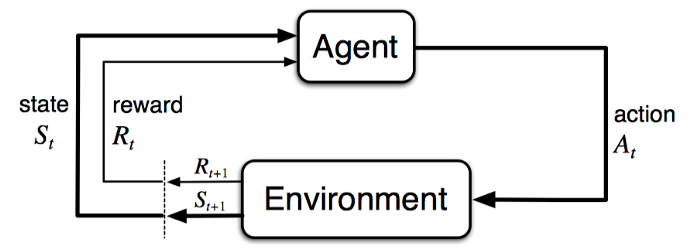
Reinforcement Learning is the most general description of the learning problem where the aim is to maximize a long-term objective. The system description consists of an agent which interacts with the environment via its actions at discrete time steps and receives a reward. This transitions the agent into a new state. A canonical agent-environment feedback loop is depicted by the figure below.
The Reinforcement Learning flavor of the learning problem is strikingly similar to how humans effectively behave — experience the world, accumulate knowledge and use the learnings to handle novel situations. Like many people, this attractive nature (although a harder formulation) of the problem is what excites me and hope it does you as well.
Policy Gradients
The objective of a Reinforcement Learning agent is to maximize the “expected” reward when following a policy π. Like any Machine Learning setup, we define a set of parameters θ (e.g. the coefficients of a complex polynomial or the weights and biases of units in a neural network) to parametrize this policy — π_θ (also written a π for brevity). If we represent the total reward for a given trajectory τ as r(τ), we arrive at the following definition.
Reinforcement Learning Objective: Maximize the “expected” reward following a parametrized policy

All finite MDPs have at least one optimal policy (which can give the maximum reward) and among all the optimal policies at least one is stationary and deterministic.
Like any other Machine Learning problem, if we can find the parameters θ⋆ which maximize J, we will have solved the task. A standard approach to solving this maximization problem in Machine Learning Literature is to use Gradient Ascent (or Descent). In gradient ascent, we keep stepping through the parameters using the following update rule

Here comes the challenge, how do we find the gradient of the objective above which contains the expectation. Integrals are always bad in a computational setting. We need to find a way around them. First step is to reformulate the gradient starting with the expansion of expectation (with a slight abuse of notation).

The Policy Gradient Theorem: The derivative of the expected reward is the expectation of the product of the reward and gradient of the log of the policy π_θ.

Now, let us expand the definition of π_θ(τ).

To understand this computation, let us break it down — P represents the ergodic distribution of starting in some state s_0. From then onwards, we apply the product rule of probability because each new action probability is independent of the previous one (remember Markov?). At each step, we take some action using the policy π_θ and the environment dynamics p decide which new state to transition into. Those are multiplied over T time steps representing the length of the trajectory. Equivalently, taking the log, we have
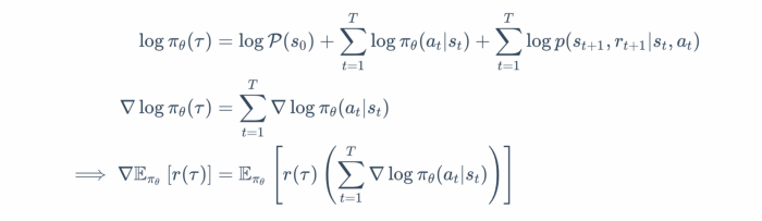
This result is beautiful in its own right because this tells us, that we don’t really need to know about the ergodic distribution of states P nor the environment dynamics p. This is crucial because for most practical purposes, it hard to model both these variables. Getting rid of them, is certainly good progress. As a result, all algorithms that use this result are known as “Model-Free Algorithms” because we don’t “model” the environment.
The “expectation” (or equivalently an integral term) still lingers around. A simple but effective approach is to sample a large number of trajectories (I really mean LARGE!) and average them out. This is an approximation but an unbiased one, similar to approximating an integral over continuous space with a discrete set of points in the domain. This technique is formally known as Markov Chain Monte-Carlo (MCMC), widely used in Probabilistic Graphical Models and Bayesian Networks to approximate parametric probability distributions.
One term that remains untouched in our treatment above is the reward of the trajectory r(τ). Even though the gradient of the parametrized policy does not depend on the reward, this term adds a lot of variance in the MCMC sampling. Effectively, there are T sources of variance with each R_t contributing. However, we can instead make use of the returns G_t because from the standpoint of optimizing the RL objective, rewards of the past don’t contribute anything. Hence, if we replace r(τ) by the discounted return G_t, we arrive at the classic algorithm Policy Gradient algorithm called REINFORCE.